RUC Land Surface Model

Description

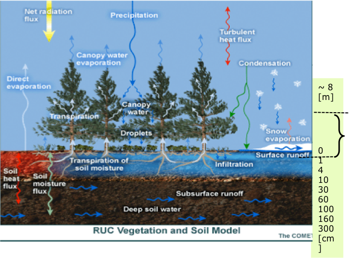
The land surface model (LSM) was originally developed as part of the NOAA Rapid Update Cycle (RUC) model development effort; with ongoing modifications, it is now used as an option for the WRF community model. The RUC model and its WRF-based NOAA successor, the Rapid Refresh (RAP) and High-Resolution Rapid Refresh (HRRR), are hourly updated and have an emphasis on short-range, near-surface forecasts including aviation-impact variables and pre-convective environment. Therefore, coupling to this LSM (hereafter the RUC LSM) has been critical to provide more accurate lower boundary conditions.

The RUC LSM became operational at the NOAA/National Centers for Environmental Prediction (NCEP) first, as part of the RUC from 1998–2012, and then as part of the RAP from 2012 through the present and as part of HRRR from 2014 through the present. The simple treatments of basic land surface processes in the RUC LSM (Smirnova et al. 2016 [182] ) have proven to be physically robust and capable of realistically representing the evolution of soil moisture, soil temperature, and snow in cycled models. Extension of the RAP domain to encompass all of North America and adjacent high-latitude ocean areas necessitated further development of the RUC LSM for application in the tundra permafrost regions and over Arctic sea ice (Smirnova et al. 2000 [181]). Other modifications include refinements in the snow model (snow "mosaic" approach, improvements in computation of snow cover fraction and snow thermal conductivity) and a more accurate specification of albedo, roughness length, and other surface properties. Some of these modifications in the RUC LSM are described and evaluated in Smirnova et al. 2016 [182] .

The parameterizations in the RUC LSM describe complicated atmosphere–land surface interactions (Fig.1) in an intentionally simplified fashion to avoid excessive sensitivity to multiple uncertain surface parameters. Nevertheless, the RUC LSM, when coupled with the hourly-assimilating atmospheric model, demonstrated over years of ongoing cycling (Benjamin et al. 2004a,b [22] [23] ; Berbery et al. 1999 [27]) that it can produce a realistic evolution of hydrologic and time-varying soil fields (i.e., soil moisture and temperature) that cannot be directly observed over large areas, as well as the evolution of snow cover on the ground surface. This result is possible only if the soil–vegetation–snow component of the coupled model, constrained only by atmospheric boundary conditions and the specification of surface characteristics, has sufficient skill to avoid long-term drift.

International projects for intercomparison of land surface and snow parameterization schemes were essential in providing the testing environment and afforded an excellent opportunity to evaluate the RUC LSM with different land use and soil types and within a variety of climates. The RUC LSM was included in phase 2(d) of the Project for the Intercomparison of Land Surface Prediction Schemes [PILPS-2(d)], in which tested models performed 18-yr simulations of the land surface state for the Valdai site in Russia (Schlosser et al. 1997 [175] ; Slater et al. 2001 [179] ;  Luo et al. 2003 [129] ). The RUC LSM was also tested during the Snow Models Intercomparison Project (SnowMIP, SnowMIP2, ESM-SnowMIP), with emphasis on snow parameterizations for both grassland and forest locations in different parts of the world (Etchevers et al. 2002, 2004 [197] [60]; Essery et al. 2009 [58] ; Rutter et al. 2009 [171] , Krinner et al. 2018 [113] ). The analysis of RUC LSM performance over 10 reference sites in ESM-SnowMIP rated it 4th place among the 26 participating models. The results were published in Menard et al.(2021) [137] and Essery et al. (2020) [59]. RUC LSM received high rankings in ESM-SnowMIP experiement in terms of multi-year snow cover and surface temperature simulations for several sites located in different parts of the world (Fig.2, Menard et al.2021 [137]).

RUC LSM is used in several weather prediction models around the world (Austria, New Zealand, Switzerland, RAP/HRRR in US). Recent RUC LSM implementation in the 1km-resolution model over Europe revealed some issues in the snow-covered high terrain (Swiss Alps), and this led to some small modifications and adjustments to the snow model. These adjustments are available in the current CCPP public release.

Coupling of the RUC LSM to physically-based stochastic snow model (He et al.(2021) [172]) is also available in the current public release.

The sensitivity of surface fluxes and turbine-height winds to the RUC LSM parameters has been explored by Geng Xia, NREL to determine the uncertainty range for the selected parameters in the RUC LSM.

RUC LSM characteristics that differ from Noah LSM:

Figure 1: RUC LSM Vegetation and Soil Model (Courtesy of T.G. Smirnova)

Figure 2: Model ranking as a function of normalized root mean square error of snow water equivalent and surface temperature (Courtesy of C. Menard)

• Implicit solution of energy and moisture budgets in the layer spanning the ground surface
• 9 soil levels with high vertical resolution near surface RUC LSM has more levels in soil than GFS Noah Land Surface Model model with higher resolution near the interface with the atmosphere
• Prognostic soil moisture variable ( \(\theta-\theta_r\)) The prognostic variables for soil moisture is volumetric soil moisture content minus residual value of soil moisture which is tied to soil particles and does not participate in moisture transport.
• Frozen soil physics algorithm RUC LSM has a different approach to take into account freezing and thawing processes in soil.
• Treatment of mixed phase precipitation accounts for mixed phase precipitation provided by Thompson Aerosol-Aware Cloud Microphysics Scheme used in RAP and HRRR.
• Simple treatment of sea ice which solves heat diffusion in sea ice and allows evolving snow cover on top of sea ice
• Sub-grid-scale heterogeneity of surface parameters in RUC LSM (Fig.3). With the certain level of confidence in the skill of the model, the next requirement is to provide land static fields and surface parameters with the best possible accuracy. RAP and HRRR use the same soil/vegetation calssifications as GFS Noah Land Surface Model. But in addition to specifying surface parameters for the dominant soil and land-use category in the grid box, RUC LSM has an option to take into account the sub-grid scale heterogeneity in the computation of such parameters as roughness length, emissivity, soil porosity, soil heat capacity and others. The difference in roughness between the mosaic and dominant category presented on Figure 3, is positive from contribution of the forests, which helped to reduce high biases of surface wind speeds in these regions. In cropland regions, roughness length also has a seasonal variability depending on the growing phase of the plants. This again helped to improve the wind forecasts during the warm season. Turning on sub-grid-scale heterogeneity option requries: mosaic_lu = 1 and mosaic_soil = 1 in the namelist, and fractions of soil and vegetation types in a grid cell.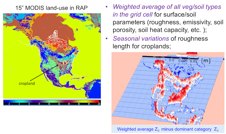
  

  Figure 3: sub-grid scale heterogeneity of surface parameters in RUC LSM (Courtesy of T.G. Smirnova)
• New: simple irrigation in the cropland area with mosaic_lu = 1
• New: water/snow intercepted by canopy as function of vegetation fraction and leaf area index (LAI)

RUC snow model characteristics:

Snow forms additional two layers on top of soil in RUC LSM

• 2-layer snow model: when SWE < 1.6 cm - snow layer is combined with top soil layer;
• Fractional snow cover (SWE < 3 cm);
• Weighted average of snow-covered and snow-free areas to compute snow parameters (roughness, albedo);
• "Mosaic" approach for patchy snow (Fig.4):
  • Separate treatment of energy and moisture budgets for snow-covered and snow-free portions of the grid cell
  • Aggregate solutions at the end of time step
  • Outcome: reduced cold bias for areas with thin snow
    

    Figure 4: 'Mosaic' approach for patchy snow (Courtesy of T.G. Smirnova)
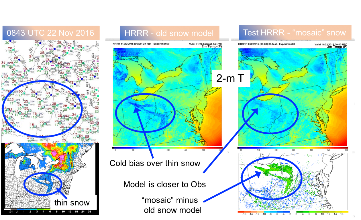
  • New: additional options to compute snow cover fraction (isncovr_opt =2 and 3, Niu and Yang (2007) [149]). These options allowed to reduce overprediction of number of grid cells fully covered with snow which further reduced cold-biases over snow. Figure 5 demonstrates that option 3 of snow cover fraction computation (isncovr_opt = 3) in the UFS-based regional model matches better the satellite data for the test case on 6 February 2022.
• New: added an option to use of a new formulation of snow thermal conductivity (isncond_opt = 2, Sturm et al. (1997) [185]);
  

  Figure 5: Snow cover fraction from MODIS (a,b), Regional UFS-based system (RRFS) original (c), and modified with isncover_opt=3 (d), 6 February 2022. (Courtesy of T.G. Smirnova)
• Iterative snow melting algorithm;
• Density of snow on the ground - a function of compaction parameter and snow depth and temperature;
• Snow albedo - a function of temperature and snow fraction;
• Snow interception by canopy - a function of vegetation fraction and leaf area index (LAI);
• Density of falling snow/graupel/ice precipitation (Fig.6)
  • The density of falling snow/graupel/ice is computed inside RUC LSM using empirical temperature-dependent equations;
  • Averaged density of frozen precipitation is defined from weighted contribution of each hydrometeor species:

    \[ \rho_{fr}=\rho_{sn}*\alpha_{sn}+\rho_{gr}*\alpha_{gr}+\rho_{ice}*\alpha_{ice} \]

    Where subscripts sn, gr, ice - snow, graupel and ice precipitation, respectively.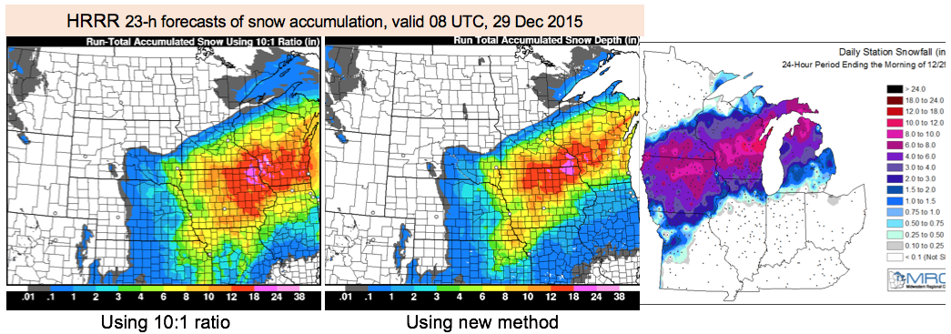
• The depth of new snow is defined from its liquid equivalent and \(\rho_{fr}\)
  

  Figure 6: HRRR 23-h forecasts of snow accumulation, valid 08 UTC, 29 Dec 2015 (Courtesy of T.G. Smirnova)

Snow accumulation with variable density is provided as an additional product in the model guidance. Figure 6 shows one example of this product from the 23-h HRRR forecast for snowstorm on 29 Dec 2015. This product is in the middle panel. The panel on the left uses traditional 10:1 ratio, and the right panel is observed snow accumulation. We can see that the new product in the middle here has a better, further north location of maximum snow accumulation, and high amounts of snow in the product with 10:1 ratio are trimmed in central and southern Iowa where both observed and model precipitation had a high content of sleet. There is even larger improvement in the Chicago area, where observed and model precipitation were almost totally sleet.

Physics Updates

Version

UFS-SRW v2.2.0

• Initialization of land and ice emissivity with consideration of partial snow cover
• Initialization of land and ice albedo with consideration of partial snow cover
• Initialization of water vapor mixing ratio over land and ice
• Initialization of fractions of soil and vegetation types in a grid cell
• Changes in the computation of a flag for sea ice: it is set to true only if flag_cice = .false. (uncoupled sea ice model)
• Introduced separate variables for sea ice, for example: showfallac is replaced with snowfallac_ice
• Added accommodation of fractional surface grid (land and ice fractions are possible within the grid cell)
• Solar angle dependence of albedo for snow-free land
• SPP option for stochastic perturbations for emissivity, albedo and vegetation fraction
• Based on RRFS testing, the coefficient in the soil resistance formulation (Sakaguchi and Zeng (2009) [173]) was increased from 0.7 to 1.0 to increase soil resistance to evaporation

Intraphysics Communication

• Argument Table

General Algorithm

• module_sf_ruclsm::lsmruc