|
CCPP SciDoc for UFS-SRW v3.0.0
SRW v3.0.0
Common Community Physics Package Developed at DTC
|


|
|
CCPP SciDoc for UFS-SRW v3.0.0
SRW v3.0.0
Common Community Physics Package Developed at DTC
|
|
The Community Land Model (CLM) lake model is a multi-level one-dimensional lake model that has been implemented within the operational 3-km HRRR and 13-km RAP for small lakes (Benjamin et al. (2022) [26]). It is the Community Land Model, version 4.5. Subin et al. (2012) [186] describe the 1-d CLM lake model as applied within the Community Earth System Model (CESM) as a component of the overall CESM CLM (Lawrence et al. (2019) [115]). Gu et al. (2015) [78] describe the introduction of the CLM lake model into the WRF model and inital experiments using its 1-d solution for both lakes Superior (average depth of 147 m) and Erie (average depth of 19 m).
The atmospheric inputs into the model are temperature, water vapor, horizontal wind components from the lowest atmospheric level and short-wave and longwave radiative fluxes. The CLM lake model then provides latent heat and sensible heat fluxes back to the atmosphere. It also computes 2-m temperature/moisture, skin temperature, lake temperature, ice fraction, ice thickness, snow water equivalent and snow depth. The CLM lake model divides the vertical lake profile into 10 layers driven by wind-driven eddies. The thickness of the top layer is fixed to 10-cm and the rest of the lake depth is divided evenly into the other 9 layers. Energy transfer (heat and kinetic energy) occurs between lake layers via eddy and molecular diffusion as a function of the vertical temperature gradient. The CLM lake model also uses a 10-layer soil model beneath the lake, a multi-layer ice formation model and up to 5-layer snow-on-ice model. Multiple layers in lake model have the potential to better represent vertical mixing processes in the lake.
Testing of the CLM lake model within RAP/HRRR applications showed computational efficiency of the model with no change of even 0.1% in run time. The lake/snow variables have to be continuously transfered within the CLM lake model from one forecast to another, constrained by the atmospheric data assimilation. The lake-cycling initialization in RAP/HRRR has been effective overall, owing to accurate houly estimates of near-surface temperature, moisture and winds, and shortwave and longwave estimates provided to the 1-d CLM lake model every time step (Benjamin et al. (2022) [26]). Cycling technique showed improvements over initializing lake temperatures from the SST analysis, problematic for small water bodies. The improvements are particularly eminent during transition periods between cold and warm seasons, and in the regions with anomalies in weather conditions. The CLM lake model has the potential to improve surface prediction in the vicinity of small lakes.
The CLM lake model requires bathymetry for the lake points in the model domain. Grid points are assigned as lake points when the fraction of lake coverage in the grid cell exceeds 50% and when this point is disconnected from oceans. The lake water mask is therefore binary, set to either 1 or 0. This binary approach for models with higher horizontal resolution, for example, 3-km resolution in in the UFS SRW App, is capable of capturing the effect of lakes on regional heat and moisture fluxes.
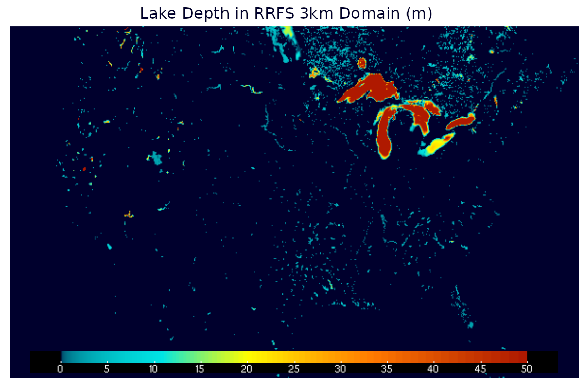
Lake depths for the RRFS lake configuration (Fig.1) are assigned from a global dataset provided by Kourzeneva et al.(2012) [112], this dataset is referred to as GLOBv3 bathymetry in the UFS_UTL.
To cold-start the CLM lake model in the UFS SRW App:
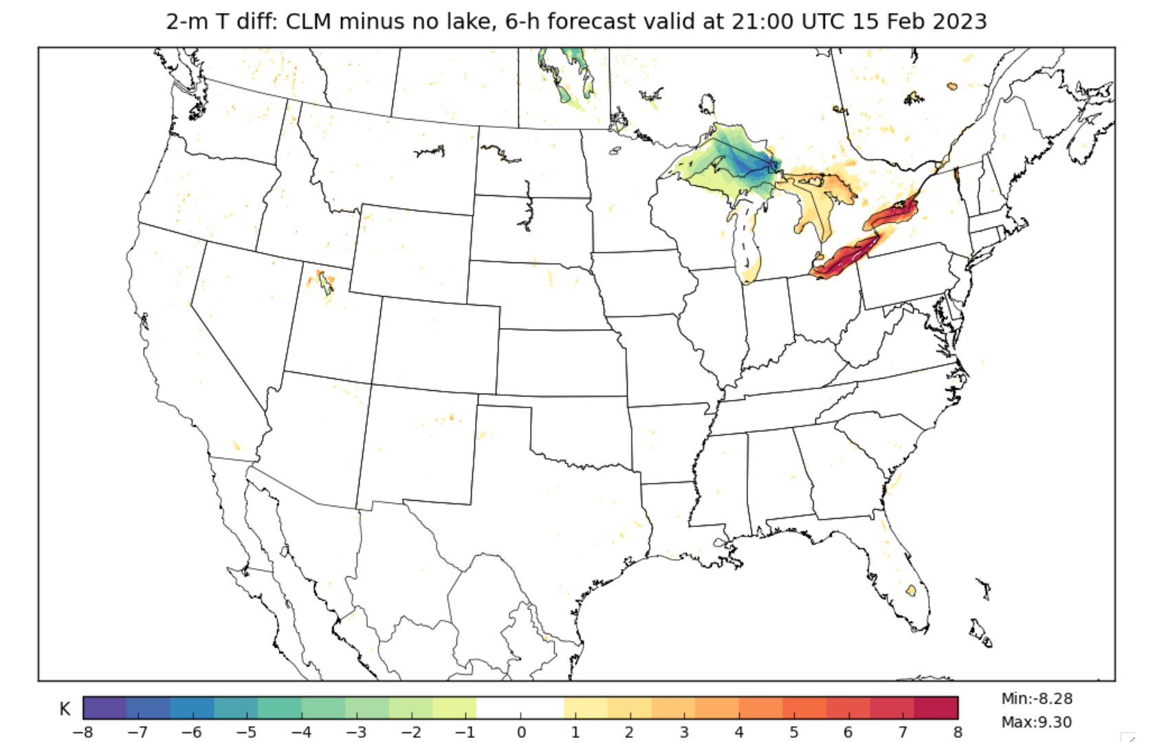
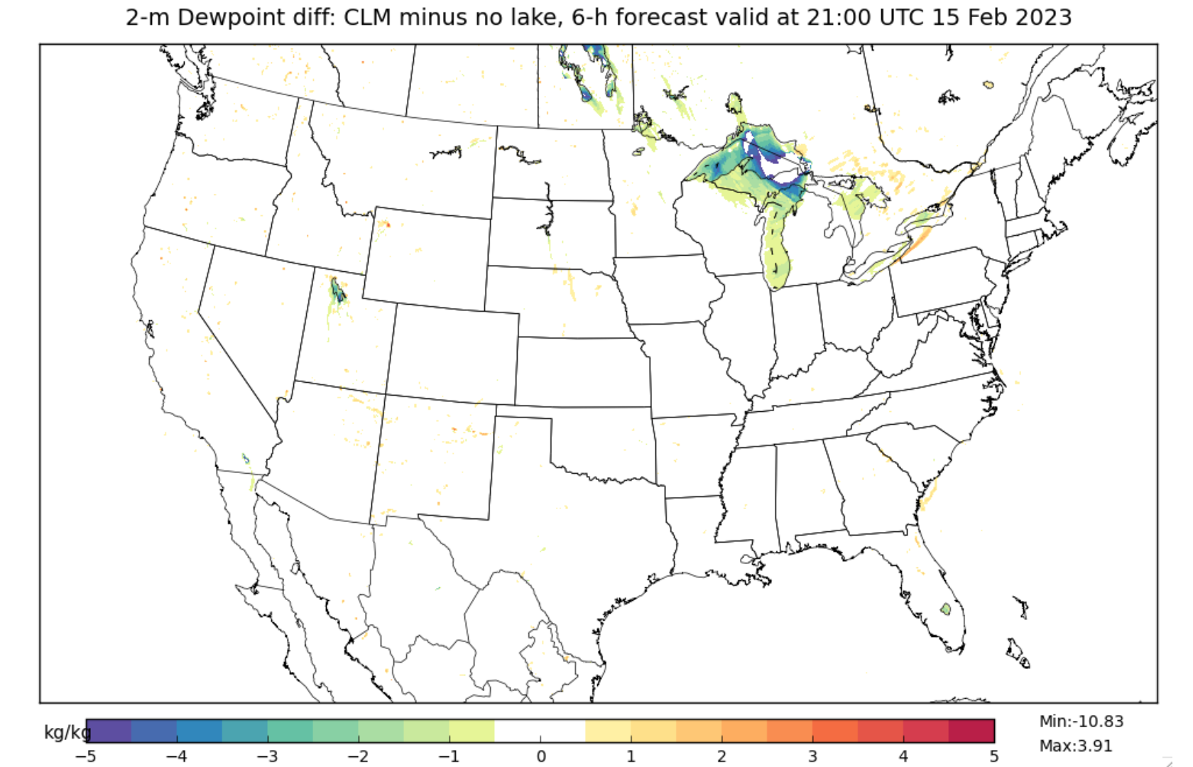
The differences of surface variables from the experimental RRFS 6-h forecast with/without CLM lake model are shown in Figure 2 for 2-m temperature and in Figure 3 for 2-m dewpoint.