The Simplified Arakawa-Schubert scheme parameterizes the effect of deep convection on the environment (represented by the model state variables) in the following way. First, a simple cloud model is used to determine the change in model state variables due to one entraining/detraining cloud type, per unit cloud-base mass flux. Next, the total change in state variables is retrieved by determining the actual cloud base mass flux using the quasi-equilibrium assumption, whereby convection is assumed to be steady-state. This implies that the generation of the cloud work function (interpreted as entrainment-moderated convective available potential energy (CAPE)) by the large scale dynamics is in balance with the consumption of the cloud work function by the convection. More...

Detailed Description

The Simplified Arakawa-Schubert scheme parameterizes the effect of deep convection on the environment (represented by the model state variables) in the following way. First, a simple cloud model is used to determine the change in model state variables due to one entraining/detraining cloud type, per unit cloud-base mass flux. Next, the total change in state variables is retrieved by determining the actual cloud base mass flux using the quasi-equilibrium assumption, whereby convection is assumed to be steady-state. This implies that the generation of the cloud work function (interpreted as entrainment-moderated convective available potential energy (CAPE)) by the large scale dynamics is in balance with the consumption of the cloud work function by the convection.

The SAS scheme uses the working concepts put forth in Arakawa and Schubert (1974) [2] but includes modifications and simplifications from Grell (1993) [21] such as saturated downdrafts and only one cloud type (the deepest possible), rather than a spectrum based on cloud top heights or assumed entrainment rates. The scheme was implemented for the GFS in 1995 by Pan and Wu [47], with further modifications discussed in Han and Pan (2011) [23] , including the calculation of cloud top, a greater CFL-criterion-based maximum cloud base mass flux, updated cloud model entrainment and detrainment, improved convective transport of horizontal momentum, a more general triggering function, and the inclusion of convective overshooting.

Calling Hierarchy Diagram

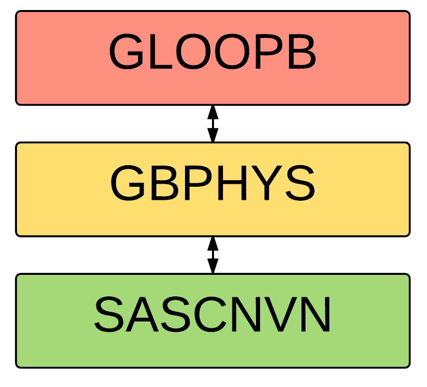
Diagram depicting how the SAS deep convection scheme is called from the GSM physics time loop

Intraphysics Communication

This space is reserved for a description of how this scheme uses information from other scheme types and/or how information calculated in this scheme is used in other scheme types.

Files
file	sascnvn.f
	Contains the entire SAS deep convection scheme.

subroutine	sascnvn (im, ix, km, jcap, delt, delp, prslp, psp, phil, ql, q1, t1, u1, v1, cldwrk, rn, kbot, ktop, kcnv, islimsk, dot, ncloud, ud_mf, dd_mf, dt_mf, cnvw, cnvc)
	This subroutine contains the entirety of the SAS deep convection scheme. More...

Function/Subroutine Documentation

subroutine sascnvn	(	integer	im,
		integer	ix,
		integer	km,
		integer	jcap,
		real(kind=kind_phys)	delt,
		real(kind=kind_phys), dimension(ix,km)	delp,
		real(kind=kind_phys), dimension(ix,km)	prslp,
		real(kind=kind_phys), dimension(im)	psp,
		real(kind=kind_phys), dimension(ix,km)	phil,
		real(kind=kind_phys), dimension(ix,km,2)	ql,
		real(kind=kind_phys), dimension(ix,km)	q1,
		real(kind=kind_phys), dimension(ix,km)	t1,
		real(kind=kind_phys), dimension(ix,km)	u1,
		real(kind=kind_phys), dimension(ix,km)	v1,
		real(kind=kind_phys), dimension(im)	cldwrk,
		real(kind=kind_phys), dimension(im)	rn,
		integer, dimension(im)	kbot,
		integer, dimension(im)	ktop,
		integer, dimension(im)	kcnv,
		integer, dimension(im), intent(in)	islimsk,
		real(kind=kind_phys), dimension(ix,km)	dot,
		integer	ncloud,
		real(kind=kind_phys), dimension(im,km)	ud_mf,
		real(kind=kind_phys), dimension(im,km)	dd_mf,
		real(kind=kind_phys), dimension(im,km)	dt_mf,
		real(kind=kind_phys), dimension(ix,km)	cnvw,
		real(kind=kind_phys), dimension(ix,km)	cnvc
	)

This subroutine contains the entirety of the SAS deep convection scheme.

As in Grell (1993) [21] , the SAS convective scheme can be described in terms of three types of "controls": static, dynamic, and feedback. The static control component consists of the simple entraining/detraining updraft/downdraft cloud model and is used to determine the cloud properties, convective precipitation, as well as the convective cloud top height. The dynamic control is the determination of the potential energy available for convection to "consume", or how primed the large-scale environment is for convection to occur due to changes by the dyanmics of the host model. The feedback control is the determination of how the parameterized convection changes the large-scale environment (the host model state variables) given the changes to the state variables per unit cloud base mass flux calculated in the static control portion and the deduced cloud base mass flux determined from the dynamic control.

Parameters

[in]	im	number of used points
[in]	ix	horizontal dimension
[in]	km	vertical layer dimension
[in]	jcap	number of spectral wave trancation
[in]	delt	physics time step in seconds
[in]	delp	pressure difference between level k and k+1 (Pa)
[in]	prslp	mean layer presure (Pa)
[in]	psp	surface pressure (Pa)
[in]	phil	layer geopotential ( \(m^2/s^2\))
[in,out]	ql	cloud water or ice (kg/kg)
[in,out]	q1	updated tracers (kg/kg)
[in,out]	t1	updated temperature (K)
[in,out]	u1	updated zonal wind ( \(m s^{-1}\))
[in,out]	v1	updated meridional wind ( \(m s^{-1}\))
[out]	cldwrk	cloud workfunction ( \(m^2/s^2\))
[out]	rn	convective rain (m)
[out]	kbot	index for cloud base
[out]	ktop	index for cloud top
[out]	kcnv	flag to denote deep convection (0=no, 1=yes)
[in]	islimsk	sea/land/ice mask (=0/1/2)
[in]	dot	layer mean vertical velocity (Pa/s)
[in]	ncloud	number of cloud species
[out]	ud_mf	updraft mass flux multiplied by time step ( \(kg/m^2\))
[out]	dd_mf	downdraft mass flux multiplied by time step ( \(kg/m^2\))
[out]	dt_mf	ud_mf at cloud top ( \(kg/m^2\))
[out]	cnvw	convective cloud water (kg/kg)
[out]	cnvc	convective cloud cover (unitless)

General Algorithm

Compute preliminary quantities needed for static, dynamic, and feedback control portions of the algorithm.
Perform calculations related to the updraft of the entraining/detraining cloud model ("static control").
Perform calculations related to the downdraft of the entraining/detraining cloud model ("static control").
Using the updated temperature and moisture profiles that were modified by the convection on a short time-scale, recalculate the total cloud work function to determine the change in the cloud work function due to convection, or the stabilizing effect of the cumulus.
For the "dynamic control", using a reference cloud work function, estimate the change in cloud work function due to the large-scale dynamics. Following the quasi-equilibrium assumption, calculate the cloud base mass flux required to keep the large-scale convective destabilization in balance with the stabilization effect of the convection.
For the "feedback control", calculate updated values of the state variables by multiplying the cloud base mass flux and the tendencies calculated per unit cloud base mass flux from the static control.

Detailed Algorithm

Compute preliminary quantities needed for static, dynamic, and feedback control portions of the algorithm.

Convert input pressure terms to centibar units.
Initialize column-integrated and other single-value-per-column variable arrays.
Initialize convective cloud water and cloud cover to zero.
Initialize updraft, downdraft, detrainment mass fluxes to zero.
Initialize the reference cloud work function, define min/max convective adjustment timescales, and tunable parameters.
Determine maximum indices for the parcel starting point (kbm), LFC (kbmax), and cloud top (kmax).
Calculate hydrostatic height at layer centers assuming a flat surface (no terrain) from the geopotential.
Calculate interface height and the initial entrainment rate as an inverse function of height.
Convert prsl from centibar to millibar, set normalized mass fluxes to 1, cloud properties to 0, and save model state variables (after advection/turbulence).
Calculate saturation mixing ratio and enforce minimum moisture values.
Calculate moist static energy (heo) and saturation moist static energy (heso).

Perform calculations related to the updraft of the entraining/detraining cloud model ("static control").

Search below index "kbm" for the level of maximum moist static energy.
Calculate the temperature, water vapor mixing ratio, and pressure at interface levels.
Recalculate saturation mixing ratio, moist static energy, saturation moist static energy, and horizontal momentum on interface levels. Enforce minimum mixing ratios and calculate \((1 - RH)\).
Search below the index "kbmax" for the level of free convection (LFC) where the condition \(h_b > h^*\) is first met, where \(h_b, h^*\) are the state moist static energy at the parcel's starting level and saturation moist static energy, respectively. Set "kbcon" to the index of the LFC.
If no LFC, return to the calling routine without modifying state variables.
Determine the vertical pressure velocity at the LFC. After Han and Pan (2011) [23] , determine the maximum pressure thickness between a parcel's starting level and the LFC. If a parcel doesn't reach the LFC within the critical thickness, then the convective inhibition is deemed too great for convection to be triggered, and the subroutine returns to the calling routine without modifying the state variables.
Calculate the entrainment rate according to Han and Pan (2011) [23] , equation 8, after Bechtold et al. (2008) [5], equation 2 given by:
\[ \epsilon = \epsilon_0F_0 + d_1\left(1-RH\right)F_1 \]
where \(\epsilon_0\) is the cloud base entrainment rate, \(d_1\) is a tunable constant, and \(F_0=\left(\frac{q_s}{q_{s,b}}\right)^2\) and \(F_1=\left(\frac{q_s}{q_{s,b}}\right)^3\) where \(q_s\) and \(q_{s,b}\) are the saturation specific humidities at a given level and cloud base, respectively. The detrainment rate in the cloud is assumed to be equal to the entrainment rate at cloud base.
The updraft detrainment rate is set constant and equal to the entrainment rate at cloud base.
Calculate the normalized mass flux for subcloud and in-cloud layers according to Pan and Wu (1995) [47] equation 1:
\[ \frac{1}{\eta}\frac{\partial \eta}{\partial z} = \lambda_e - \lambda_d \]
where \(\eta\) is the normalized mass flux, \(\lambda_e\) is the entrainment rate and \(\lambda_d\) is the detrainment rate.
Set initial cloud properties equal to the state variables at cloud base.
Calculate the cloud properties as a parcel ascends, modified by entrainment and detrainment. Discretization follows Appendix B of Grell (1993) [21] . Following Han and Pan (2006) [22], the convective momentum transport is reduced by the convection-induced pressure gradient force by the constant "pgcon", currently set to 0.55 after Zhang and Wu (2003) [63] .
With entrainment, recalculate the LFC as the first level where buoyancy is positive. The difference in pressure levels between LFCs calculated with/without entrainment must be less than a threshold (currently 25 hPa). Otherwise, convection is inhibited and the scheme returns to the calling routine without modifying the state variables. This is the subcloud dryness trigger modification discussed in Han and Pan (2011) [23].
Calculate the cloud top as the first level where parcel buoyancy becomes negative. If the thickness of the calculated convection is less than a threshold (currently 150 hPa), then convection is inhibited, and the scheme returns to the calling routine.
To originate the downdraft, search for the level above the minimum in moist static energy. Return to the calling routine without modification if this level is determined to be outside of the convective cloud layers.
Calculate the maximum value of the cloud base mass flux using the CFL-criterion-based formula of Han and Pan (2011) [23], equation 7.
Initialize the cloud moisture at cloud base and set the cloud work function to zero.
Calculate the moisture content of the entraining/detraining parcel (qcko) and the value it would have if just saturated (qrch), according to equation A.14 in Grell (1993) [21] . Their difference is the amount of convective cloud water (qlk = rain + condensate). Determine the portion of convective cloud water that remains suspended and the portion that is converted into convective precipitation (pwo). Calculate and save the negative cloud work function (aa1) due to water loading. The liquid water in the updraft layer is assumed to be detrained from the layers above the level of the minimum moist static energy into the grid-scale cloud water (dellal).
Calculate the cloud work function according to Pan and Wu (1995) [47] equation 4:
\[ A_u=\int_{z_0}^{z_t}\frac{g}{c_pT(z)}\frac{\eta}{1 + \gamma}[h(z)-h^*(z)]dz \]
(discretized according to Grell (1993) [21] equation B.10 using B.2 and B.3 of Arakawa and Schubert (1974) [2] and assuming \(\eta=1\)) where \(A_u\) is the updraft cloud work function, \(z_0\) and \(z_t\) are cloud base and cloud top, respectively, \(\gamma = \frac{L}{c_p}\left(\frac{\partial \overline{q_s}}{\partial T}\right)_p\) and other quantities are previously defined.
If the updraft cloud work function is negative, convection does not occur, and the scheme returns to the calling routine.
Continue calculating the cloud work function past the point of neutral buoyancy to represent overshooting according to Han and Pan (2011) [23] . Convective overshooting stops when \( cA_u < 0\) where \(c\) is currently 10%, or when 10% of the updraft cloud work function has been consumed by the stable buoyancy force.
For the overshooting convection, calculate the moisture content of the entraining/detraining parcel as before. Partition convective cloud water and precipitation and detrain convective cloud water above the mimimum in moist static energy.
Swap the indices of the convective cloud top (ktcon) and the overshooting convection top (ktcon1) to use the same cloud top level in the calculations of \(A^+\) and \(A^*\).
Separate the total updraft cloud water at cloud top into vapor and condensate.

Perform calculations related to the downdraft of the entraining/detraining cloud model ("static control").

First, in order to calculate the downdraft mass flux (as a fraction of the updraft mass flux), calculate the wind shear and precipitation efficiency according to equation 58 in Fritsch and Chappell (1980) [16] :
\[ E = 1.591 - 0.639\frac{\Delta V}{\Delta z} + 0.0953\left(\frac{\Delta V}{\Delta z}\right)^2 - 0.00496\left(\frac{\Delta V}{\Delta z}\right)^3 \]
where \(\Delta V\) is the integrated horizontal shear over the cloud depth, \(\Delta z\), (the ratio is converted to units of \(10^{-3} s^{-1}\)). The variable "edto" is \(1-E\) and is constrained to the range \([0,0.9]\).
Next, calculate the variable detrainment rate between the surface and the LFC according to:
\[ \lambda_d = \frac{1-\beta^{\frac{1}{k_{LFC}}}}{\overline{\Delta z}} \]
\(\lambda_d\) is the detrainment rate, \(\beta\) is a constant currently set to 0.05, \(k_{LFC}\) is the vertical index of the LFC level, and \(\overline{\Delta z}\) is the average vertical grid spacing below the LFC.
Calculate the normalized downdraft mass flux from equation 1 of Pan and Wu (1995) [47] . Downdraft entrainment and detrainment rates are constants from the downdraft origination to the LFC.
Set initial cloud downdraft properties equal to the state variables at the downdraft origination level.
Calculate the cloud properties as a parcel descends, modified by entrainment and detrainment. Discretization follows Appendix B of Grell (1993) [21] .
Compute the amount of moisture that is necessary to keep the downdraft saturated.
Update the precipitation efficiency (edto) based on the ratio of normalized cloud condensate (pwavo) to normalized cloud evaporate (pwevo).
Calculate downdraft cloud work function ( \(A_d\)) according to equation A.42 (discretized by B.11) in Grell (1993) [21] . Add it to the updraft cloud work function, \(A_u\).
Check for negative total cloud work function; if found, return to calling routine without modifying state variables.
Calculate the change in moist static energy, moisture mixing ratio, and horizontal winds per unit cloud base mass flux near the surface using equations B.18 and B.19 from Grell (1993) [21], for all layers below cloud top from equations B.14 and B.15, and for the cloud top from B.16 and B.17.
Calculate the change in the temperature and moisture profiles per unit cloud base mass flux.

Using the updated temperature and moisture profiles that were modified by the convection on a short time-scale, recalculate the total cloud work function to determine the change in the cloud work function due to convection, or the stabilizing effect of the cumulus.

Using notation from Pan and Wu (1995) [47], the previously calculated cloud work function is denoted by \(A^+\). Now, it is necessary to use the entraining/detraining cloud model ("static control") to determine the cloud work function of the environment after the stabilization of the arbitrary convective element (per unit cloud base mass flux) has been applied, denoted by \(A^*\).
Recalculate saturation specific humidity.
As before, recalculate the updraft cloud work function.
As before, recalculate the downdraft cloud work function.

For the "dynamic control", using a reference cloud work function, estimate the change in cloud work function due to the large-scale dynamics. Following the quasi-equilibrium assumption, calculate the cloud base mass flux required to keep the large-scale convective destabilization in balance with the stabilization effect of the convection.

Calculate the reference, or "critical", cloud work function derived from observations, denoted by \(A^0\).
Calculate a correction factor, "acrtfct", that is a function of the cloud base vertical velocity, to multiply the critical cloud work function.
Also, modify the time scale over which the large-scale destabilization takes place (dtconv) according to the cloud base vertical velocity, ensuring that this timescale stays between previously calculated minimum and maximum values.
Calculate the large scale destabilization as in equation 5 of Pan and Wu (1995) [47] :
\[ \frac{\partial A}{\partial t}_{LS}=\frac{A^+-cA^0}{\Delta t_{LS}} \]
where \(c\) is the correction factor "acrtfct", \(\Delta t_{LS}\) is the modified timescale over which the environment is destabilized, and the other quantities have been previously defined.
Calculate the stabilization effect of the convection (per unit cloud base mass flux) as in equation 6 of Pan and Wu (1995) [47] :
\[ \frac{\partial A}{\partial t}_{cu}=\frac{A^*-A^+}{\Delta t_{cu}} \]
\(\Delta t_{cu}\) is the short timescale of the convection.
The cloud base mass flux (xmb) is then calculated from equation 7 of Pan and Wu (1995) [47]
\[ M_c=\frac{-\frac{\partial A}{\partial t}_{LS}}{\frac{\partial A}{\partial t}_{cu}} \]
If the large scale destabilization is less than zero, or the stabilization by the convection is greater than zero, then the scheme returns to the calling routine without modifying the state variables.

For the "feedback" control, calculate updated values of the state variables by multiplying the cloud base mass flux and the tendencies calculated per unit cloud base mass flux from the static control.

Calculate the temperature tendency from the moist static energy and specific humidity tendencies.
Update the temperature, specific humidity, and horiztonal wind state variables by multiplying the cloud base mass flux-normalized tendencies by the cloud base mass flux.
Accumulate column-integrated tendencies.
Recalculate saturation specific humidity using the updated temperature.
Add up column-integrated convective precipitation by multiplying the normalized value by the cloud base mass flux.
Determine the evaporation of the convective precipitation and update the integrated convective precipitation.
Update state temperature and moisture to account for evaporation of convective precipitation.
Update column-integrated tendencies to account for evaporation of convective precipitation.
Calculate convective cloud water.
Calculate convective cloud cover.
Separate detrained cloud water into liquid and ice species as a function of temperature only.
If convective precipitation is zero or negative, reset the updated state variables back to their original values (negating convective changes).
Calculate the updraft convective mass flux.
Calculate the detrainment mass flux at cloud top.
Calculate the downdraft convective mass flux.

Definition at line 59 of file sascnvn.f.

References physcons::con_cliq, physcons::con_cp, physcons::con_cvap, physcons::con_g, physcons::con_hvap, physcons::con_rv, and physcons::con_t0c.

Referenced by gbphys().

Here is the caller graph for this function: