Description

GFDL cloud microphysics (MP) scheme is a six-category MP scheme to replace Zhao-Carr MP scheme, and moves the GFS from a total cloud water variable to five predicted hydrometeors (cloud water, cloud ice, rain, snow and graupel). This scheme utilizes the "bulk water" microphysical parameterization technique in Lin et al. (1983) [65] and has been significantly improved over years at GFDL (Lord et al.(1984) [72], Krueger et al.(1995) [61], Chen and Lin (2011) [12], Chen and Lin (2013) [13]). Physics processes of GFDL cloud MP are described in Figure 1 (also see warm_rain() and icloud()) and are feature with time-split between warm-rain (faster) and ice-phase (slower) processes (see 'conversion time scale' in gfdl_cloud_microphys.F90 for default values).

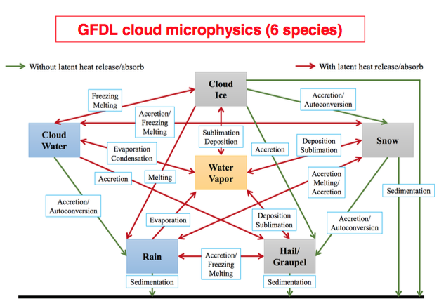
Figure 1: GFDL MP at a glance (Courtesy of S.J. Lin at GFDL)

Some unique attributes of GFDL cloud microphysics include:

Fast Physics in FV3 dynamical solver

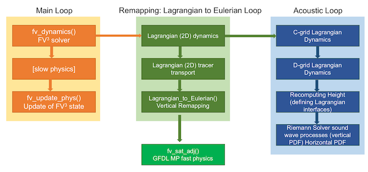
Figure 1: FV3 structure; Yellow represents external API routines, called once per physics time step; Green are called once per remapping time step; Blue are called once per acoustic time step.

The leftmost column of Figure 1 shows the external API calls used during a typical process-split model integration procedure. First, the solver is called, which advances the solver a full "physics" time step. This updated state is then passed to the physical parameterization package, which then computes the physics tendencies over the same time interval. Finally, the tendencies are then used to update the model state using a forward-in-time evaluation consistent with the dynamics.
There are two levels of time-stepping inside FV3. The first is the "remapping" loop, the green column in Figure 1. This loop has three steps:

Perform the Lagrangian dynamics, the loop shown in the blue column of Figure 1.
Perform the subcycled tracer advection along Lagrangian surfaces, using accumulated mass fluxes from the Lagrangian dynamics. Subcycling is done independently within each layer to maintain local (within each layer) stability.
Remap the deformal Lagrangian surfaces on to the reference, or "Eulerian", coordinate levels.

This loop is typically performed once per call to the solver, although it is possible to improve the model's stability by executing the loop (and thereby the vertical remapping) multiple times per solver call.

In current fv3gfs, the fast physics (phase-changes only) is called after the "Lagrangian-to-Eulerain" remapping. When GFDL MP Fast Physics is activated (fast_sat_adj=.true. in fv_core_nml block), it adjusts cloud water evaporation (cloud water $\rightarrow$ water vapor), cloud water freezing (cloud water $\rightarrow$ cloud ice), and cloud ice deposition (water vapor $\rightarrow$ cloud ice). The process of condensation is an interesting and well known example. Say dynamics lifts a column of air above saturation, then an adjustment is made to temperature and moisture in order to reach saturation. The tendency of the dynamics has been included in this procedure in order to have the correct balance.

Horizontal Sub-grid Variability ("Scale-aware")
Horizontal sub-grid variability is a function of cell area:

Over land:
$h_{var}=\min \left\{0.2,\max\left[0.01, D_{land}(\frac{A_{r}}{10^{10}})^{0.25}\right]\right\}$
Over Ocean:
$h_{var}=\min \left\{0.2,\max\left[0.01, D_{ocean}(\frac{A_{r}}{10^{10}})^{0.25}\right]\right\}$

Where $A_{r}$ is cell area, $D_{land}$ and $D_{ocean}$ are base values for sub-grid variability over land and ocean (larger sub-grid variability appears in larger area). Horizontal sub-grid variability is used in cloud fraction, relative humidity calculation, evaporation and condensation processes. Scale-awareness is achieved by this horizontal subgrid variability and a $2^{nd}$ order FV-type vertical reconstruction (Lin et al.(1994) [66]).

Intraphysics Communication

For GFDL Cloud MP: Argument Table
For GFDL Fast Physics: Argument Table

General Algorithm

For GFDL Cloud MP: mpdrv()
For GFDL Fast Physics: fv_sat_adj_work()