The Mass-Flux shallow convection scheme parameterizes the effect of shallow convection on the environment much like the Simplified Arakawa-Schubert Deep Convection scheme with a few key modifications. Perhaps most importantly, no quasi-equilibrium assumption is necessary since the shallow cloud base mass flux is parameterized from the surface buoyancy flux. Further, there are no convective downdrafts, the entrainment rate is greater than for deep convection, and the shallow convection is limited to not extend over the level where \(p=0.7p_{sfc}\). More...

Detailed Description

The Mass-Flux shallow convection scheme parameterizes the effect of shallow convection on the environment much like the Simplified Arakawa-Schubert Deep Convection scheme with a few key modifications. Perhaps most importantly, no quasi-equilibrium assumption is necessary since the shallow cloud base mass flux is parameterized from the surface buoyancy flux. Further, there are no convective downdrafts, the entrainment rate is greater than for deep convection, and the shallow convection is limited to not extend over the level where \(p=0.7p_{sfc}\).

This scheme was designed to replace the previous eddy-diffusivity approach to shallow convection with a mass-flux based approach as it is used for deep convection. Differences between the shallow and deep SAS schemes are presented in Han and Pan (2011) [23] . Like the deep scheme, it uses the working concepts put forth in Arakawa and Schubert (1974) [2] but includes modifications and simplifications from Grell (1993) [21] such as only one cloud type (the deepest possible, up to \(p=0.7p_{sfc}\)), rather than a spectrum based on cloud top heights or assumed entrainment rates, although it assumes no convective downdrafts. It contains many modifications associated with deep scheme as discussed in Han and Pan (2011) [23] , including the calculation of cloud top, a greater CFL-criterion-based maximum cloud base mass flux, and the inclusion of convective overshooting.

Calling Hierarchy Diagram

Diagram depicting how the SAS shallow convection scheme is called from the GSM physics time loop

Intraphysics Communication

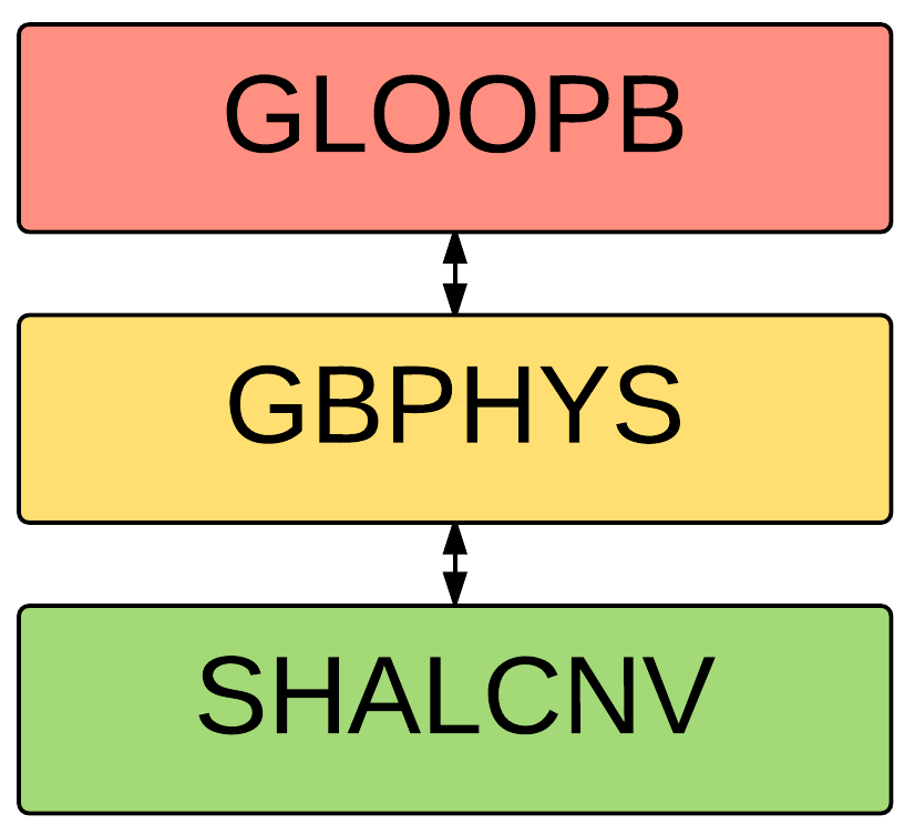
This space is reserved for a description of how this scheme uses information from other scheme types and/or how information calculated in this scheme is used in other scheme types.

Files
file	shalcnv.f
	Contains the entire SAS shallow convection scheme.

subroutine	shalcnv (im, ix, km, jcap, delt, delp, prslp, psp, phil, ql, q1, t1, u1, v1, rn, kbot, ktop, kcnv, islimsk, dot, ncloud, hpbl, heat, evap, ud_mf, dt_mf, cnvw, cnvc)
	This subroutine contains the entirety of the SAS shallow convection scheme. More...

Function/Subroutine Documentation

subroutine shalcnv	(	integer	im,
		integer	ix,
		integer	km,
		integer	jcap,
		real(kind=kind_phys)	delt,
		real(kind=kind_phys), dimension(ix,km)	delp,
		real(kind=kind_phys), dimension(ix,km)	prslp,
		real(kind=kind_phys), dimension(im)	psp,
		real(kind=kind_phys), dimension(ix,km)	phil,
		real(kind=kind_phys), dimension(ix,km,2)	ql,
		real(kind=kind_phys), dimension(ix,km)	q1,
		real(kind=kind_phys), dimension(ix,km)	t1,
		real(kind=kind_phys), dimension(ix,km)	u1,
		real(kind=kind_phys), dimension(ix,km)	v1,
		real(kind=kind_phys), dimension(im)	rn,
		integer, dimension(im)	kbot,
		integer, dimension(im)	ktop,
		integer, dimension(im)	kcnv,
		integer, dimension(im), intent(in)	islimsk,
		real(kind=kind_phys), dimension(ix,km)	dot,
		integer	ncloud,
		real(kind=kind_phys), dimension(im)	hpbl,
		real(kind=kind_phys), dimension(im)	heat,
		real(kind=kind_phys), dimension(im)	evap,
		real(kind=kind_phys), dimension(im,km)	ud_mf,
		real(kind=kind_phys), dimension(im,km)	dt_mf,
		real(kind=kind_phys), dimension(ix,km)	cnvw,
		real(kind=kind_phys), dimension(ix,km)	cnvc
	)

This subroutine contains the entirety of the SAS shallow convection scheme.

This routine follows the Simplified Arakawa-Schubert Deep Convection scheme quite closely, although it can be interpreted as only having the "static" and "feedback" control portions, since the "dynamic" control is not necessary to find the cloud base mass flux. The algorithm is simplified from SAS deep convection by excluding convective downdrafts and being confined to operate below \(p=0.7p_{sfc}\). Also, entrainment is both simpler and stronger in magnitude compared to the deep scheme.

Parameters

[in]	im	number of used points
[in]	ix	horizontal dimension
[in]	km	vertical layer dimension
[in]	jcap	number of spectral wave trancation
[in]	delt	physics time step in seconds
[in]	delp	pressure difference between level k and k+1 (Pa)
[in]	prslp	mean layer presure (Pa)
[in]	psp	surface pressure (Pa)
[in]	phil	layer geopotential ( \(m^s/s^2\))
[in,out]	ql	cloud water or ice (kg/kg)
[in,out]	q1	updated tracers (kg/kg)
[in,out]	t1	updated temperature (K)
[in,out]	u1	updated zonal wind ( \(m s^{-1}\))
[in,out]	v1	updated meridional wind ( \(m s^{-1}\))
[out]	rn	convective rain (m)
[out]	kbot	index for cloud base
[out]	ktop	index for cloud top
[out]	kcnv	flag to denote deep convection (0=no, 1=yes)
[in]	islimsk	sea/land/ice mask (=0/1/2)
[in]	dot	layer mean vertical velocity (Pa/s)
[in]	ncloud	number of cloud species
[in]	hpbl	PBL height (m)
[in]	heat	surface sensible heat flux (K m/s)
[in]	evap	surface latent heat flux (kg/kg m/s)
[out]	ud_mf	updraft mass flux multiplied by time step ( \(kg/m^2\))
[out]	dt_mf	ud_mf at cloud top ( \(kg/m^2\))
[out]	cnvw	convective cloud water (kg/kg)
[out]	cnvc	convective cloud cover (unitless)

General Algorithm

Compute preliminary quantities needed for the static and feedback control portions of the algorithm.
Perform calculations related to the updraft of the entraining/detraining cloud model ("static control").
Calculate the tendencies of the state variables (per unit cloud base mass flux) and the cloud base mass flux.
For the "feedback control", calculate updated values of the state variables by multiplying the cloud base mass flux and the tendencies calculated per unit cloud base mass flux from the static control.

Detailed Algorithm

Compute preliminary quantities needed for the static and feedback control portions of the algorithm.

Convert input pressure terms to centibar units.
Compute the surface buoyancy flux according to
\[ \overline{w'\theta_v'}=\overline{w'\theta'}+\left(\frac{R_v}{R_d}-1\right)T_0\overline{w'q'} \]
where \(\overline{w'\theta'}\) is the surface sensible heat flux, \(\overline{w'q'}\) is the surface latent heat flux, \(R_v\) is the gas constant for water vapor, \(R_d\) is the gas constant for dry air, and \(T_0\) is a reference temperature.
Initialize column-integrated and other single-value-per-column variable arrays.
Initialize updraft and detrainment mass fluxes to zero.
Return to the calling routine if deep convection is present or the surface buoyancy flux is negative.
Define tunable parameters.
Determine maximum indices for the parcel starting point (kbm) and cloud top (kmax).
Calculate hydrostatic height at layer centers assuming a flat surface (no terrain) from the geopotential.
Calculate interface height and the entrainment rate as an inverse function of height.
Find the index for the PBL top using the PBL height; enforce that it is lower than the maximum parcel starting level.
Convert prsl from centibar to millibar, set normalized mass flux to 1, cloud properties to 0, and save model state variables (after advection/turbulence).
Calculate saturation mixing ratio and enforce minimum moisture values.
Calculate moist static energy (heo) and saturation moist static energy (heso).

Perform calculations related to the updraft of the entraining/detraining cloud model ("static control").

Search in the PBL for the level of maximum moist static energy to start the ascending parcel.
Calculate the temperature, water vapor mixing ratio, and pressure at interface levels.
Recalculate saturation mixing ratio, moist static energy, saturation moist static energy, and horizontal momentum on interface levels. Enforce minimum mixing ratios.
Search below the index "kbm" for the level of free convection (LFC) where the condition \(h_b > h^*\) is first met, where \(h_b, h^*\) are the state moist static energy at the parcel's starting level and saturation moist static energy, respectively. Set "kbcon" to the index of the LFC.
If no LFC, return to the calling routine without modifying state variables.
Determine the vertical pressure velocity at the LFC. After Han and Pan (2011) [23] , determine the maximum pressure thickness between a parcel's starting level and the LFC. If a parcel doesn't reach the LFC within the critical thickness, then the convective inhibition is deemed too great for convection to be triggered, and the subroutine returns to the calling routine without modifying the state variables.
The updraft detrainment rate is set constant and equal to the entrainment rate at cloud base.
Calculate the normalized mass flux for subcloud and in-cloud layers according to Pan and Wu (1995) [47] equation 1:
\[ \frac{1}{\eta}\frac{\partial \eta}{\partial z} = \lambda_e - \lambda_d \]
where \(\eta\) is the normalized mass flux, \(\lambda_e\) is the entrainment rate and \(\lambda_d\) is the detrainment rate. The normalized mass flux increases upward below the cloud base and decreases upward above.
Set initial cloud properties equal to the state variables at cloud base.
Calculate the cloud properties as a parcel ascends, modified by entrainment and detrainment. Discretization follows Appendix B of Grell (1993) [21] . Following Han and Pan (2006) [22], the convective momentum transport is reduced by the convection-induced pressure gradient force by the constant "pgcon", currently set to 0.55 after Zhang and Wu (2003) [63] .
With entrainment, recalculate the LFC as the first level where buoyancy is positive. The difference in pressure levels between LFCs calculated with/without entrainment must be less than a threshold (currently 25 hPa). Otherwise, convection is inhibited and the scheme returns to the calling routine without modifying the state variables. This is the subcloud dryness trigger modification discussed in Han and Pan (2011) [23].
Calculate the cloud top as the first level where parcel buoyancy becomes negative; the maximum possible value is at \(p=0.7p_{sfc}\).
Calculate the maximum value of the cloud base mass flux using the CFL-criterion-based formula of Han and Pan (2011) [23], equation 7.
Initialize the cloud moisture at cloud base and set the cloud work function to zero.
Calculate the moisture content of the entraining/detraining parcel (qcko) and the value it would have if just saturated (qrch), according to equation A.14 in Grell (1993) [21] . Their difference is the amount of convective cloud water (qlk = rain + condensate). Determine the portion of convective cloud water that remains suspended and the portion that is converted into convective precipitation (pwo). Calculate and save the negative cloud work function (aa1) due to water loading. Above the level of minimum moist static energy, some of the cloud water is detrained into the grid-scale cloud water from every cloud layer with a rate of 0.0005 \(m^{-1}\) (dellal).
Calculate the cloud work function according to Pan and Wu (1995) [47] equation 4:
\[ A_u=\int_{z_0}^{z_t}\frac{g}{c_pT(z)}\frac{\eta}{1 + \gamma}[h(z)-h^*(z)]dz \]
(discretized according to Grell (1993) [21] equation B.10 using B.2 and B.3 of Arakawa and Schubert (1974) [2] and assuming \(\eta=1\)) where \(A_u\) is the updraft cloud work function, \(z_0\) and \(z_t\) are cloud base and cloud top, respectively, \(\gamma = \frac{L}{c_p}\left(\frac{\partial \overline{q_s}}{\partial T}\right)_p\) and other quantities are previously defined.
If the updraft cloud work function is negative, convection does not occur, and the scheme returns to the calling routine.
Continue calculating the cloud work function past the point of neutral buoyancy to represent overshooting according to Han and Pan (2011) [23] . Convective overshooting stops when \( cA_u < 0\) where \(c\) is currently 10%, or when 10% of the updraft cloud work function has been consumed by the stable buoyancy force. Overshooting is also limited to the level where \(p=0.7p_{sfc}\).
For the overshooting convection, calculate the moisture content of the entraining/detraining parcel as before. Partition convective cloud water and precipitation and detrain convective cloud water in the overshooting layers.
=> Separate the total updraft cloud water at cloud top into vapor and condensate.

Calculate the tendencies of the state variables (per unit cloud base mass flux) and the cloud base mass flux.

Calculate the change in moist static energy, moisture mixing ratio, and horizontal winds per unit cloud base mass flux for all layers below cloud top from equations B.14 and B.15 from Grell (1993) [21], and for the cloud top from B.16 and B.17.
Calculate the cloud base mass flux according to equation 6 in Grant (2001) [20], based on the subcloud layer convective velocity scale, \(w_*\).
\[ M_c = 0.03\rho w_* \]
where \(M_c\) is the cloud base mass flux, \(\rho\) is the air density, and \(w_*=\left(\frac{g}{T_0}\overline{w'\theta_v'}h\right)^{1/3}\) with \(h\) the PBL height and other quantities have been defined previously.

For the "feedback control", calculate updated values of the state variables by multiplying the cloud base mass flux and the tendencies calculated per unit cloud base mass flux from the static control.

Recalculate saturation specific humidity.
Calculate the temperature tendency from the moist static energy and specific humidity tendencies.
Update the temperature, specific humidity, and horiztonal wind state variables by multiplying the cloud base mass flux-normalized tendencies by the cloud base mass flux.
Accumulate column-integrated tendencies.
Recalculate saturation specific humidity using the updated temperature.
Add up column-integrated convective precipitation by multiplying the normalized value by the cloud base mass flux.
Determine the evaporation of the convective precipitation and update the integrated convective precipitation.
Update state temperature and moisture to account for evaporation of convective precipitation.
Update column-integrated tendencies to account for evaporation of convective precipitation.
Calculate shallow convective cloud water.
Calculate shallow convective cloud cover.
Separate detrained cloud water into liquid and ice species as a function of temperature only.
Calculate the updraft shallow convective mass flux.
Calculate the detrainment mass flux at shallow cloud top.

Definition at line 58 of file shalcnv.f.

References physcons::con_cliq, physcons::con_cp, physcons::con_cvap, physcons::con_g, physcons::con_hvap, physcons::con_rd, physcons::con_rv, and physcons::con_t0c.

Referenced by gbphys().

Here is the caller graph for this function: