|
GFS Operational Physics Documentation
Revision: 81451
|


|
|
GFS Operational Physics Documentation
Revision: 81451
|
|
The Hybrid EDMF scheme is a first-order turbulent transport scheme used for subgrid-scale vertical turbulent mixing in the PBL and above. It blends the traditional first-order approach that has been used and improved over the last several years with a more recent scheme that uses a mass-flux approach to calculate the countergradient diffusion terms. More...
The Hybrid EDMF scheme is a first-order turbulent transport scheme used for subgrid-scale vertical turbulent mixing in the PBL and above. It blends the traditional first-order approach that has been used and improved over the last several years with a more recent scheme that uses a mass-flux approach to calculate the countergradient diffusion terms.
The PBL scheme's main task is to calculate tendencies of temperature, moisture, and momentum due to vertical diffusion throughout the column (not just the PBL). The scheme is an amalgamation of decades of work, starting from the initial first-order PBL scheme of Troen and Mahrt (1986) [53], implemented according to Hong and Pan (1996) [26] and modified by Han and Pan (2011) [21] and Han et al. (2015) [22] to include top-down mixing due to stratocumulus layers from Lock et al. (2000) [38] and replacement of counter-gradient terms with a mass flux scheme according to Siebesma et al. (2007) [49] and Soares et al. (2004) [50]. Recently, heating due to TKE dissipation was also added according to Han et al. (2015) [22].
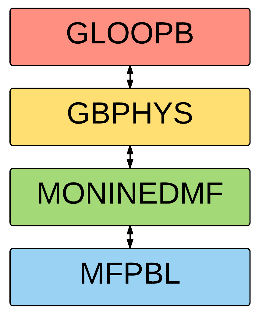
This space is reserved for a description of how this scheme uses information from other scheme types and/or how information calculated in this scheme is used in other scheme types.
Functions/Subroutines | |
| subroutine | tridi2 (l, n, cl, cm, cu, r1, r2, au, a1, a2) |
| Routine to solve the tridiagonal system to calculate temperature and moisture at \( t + \Delta t \); part of two-part process to calculate time tendencies due to vertical diffusion. More... | |
| subroutine | tridin (l, n, nt, cl, cm, cu, r1, r2, au, a1, a2) |
| Routine to solve the tridiagonal system to calculate u- and v-momentum at \( t + \Delta t \); part of two-part process to calculate time tendencies due to vertical diffusion. More... | |
| subroutine | mfpbl (im, ix, km, ntrac, delt, cnvflg, zl, zm, thvx, q1, t1, u1, v1, hpbl, kpbl, sflx, ustar, wstar, xmf, tcko, qcko, ucko, vcko) |
| This subroutine is used for calculating the mass flux and updraft properties. More... | |
| subroutine | moninedmf (ix, im, km, ntrac, ntcw, dv, du, tau, rtg, u1, v1, t1, q1, swh, hlw, xmu, psk, rbsoil, zorl, u10m, v10m, fm, fh, tsea, qss, heat, evap, stress, spd1, kpbl, prsi, del, prsl, prslk, phii, phil, delt, dspheat, dusfc, dvsfc, dtsfc, dqsfc, hpbl, hgamt, hgamq, dkt, kinver, xkzm_m, xkzm_h, xkzm_s, lprnt, ipr) |
| This subroutine contains all of logic for the Hybrid EDMF PBL scheme except for the calculation of the updraft properties and mass flux. More... | |
| subroutine mfpbl | ( | integer | im, |
| integer | ix, | ||
| integer | km, | ||
| integer | ntrac, | ||
| real(kind=kind_phys) | delt, | ||
| logical, dimension(im) | cnvflg, | ||
| real(kind=kind_phys), dimension(im,km) | zl, | ||
| real(kind=kind_phys), dimension(im,km+1) | zm, | ||
| real(kind=kind_phys), dimension(im,km) | thvx, | ||
| real(kind=kind_phys), dimension(ix,km,ntrac) | q1, | ||
| real(kind=kind_phys), dimension(ix,km) | t1, | ||
| real(kind=kind_phys), dimension(ix,km) | u1, | ||
| real(kind=kind_phys), dimension(ix,km) | v1, | ||
| real(kind=kind_phys), dimension(im) | hpbl, | ||
| integer, dimension(im) | kpbl, | ||
| real(kind=kind_phys), dimension(im) | sflx, | ||
| real(kind=kind_phys), dimension(im) | ustar, | ||
| real(kind=kind_phys), dimension(im) | wstar, | ||
| real(kind=kind_phys), dimension(im,km) | xmf, | ||
| real(kind=kind_phys), dimension(im,km) | tcko, | ||
| real(kind=kind_phys), dimension(im,km,ntrac) | qcko, | ||
| real(kind=kind_phys), dimension(im,km) | ucko, | ||
| real(kind=kind_phys), dimension(im,km) | vcko | ||
| ) |
This subroutine is used for calculating the mass flux and updraft properties.
The mfpbl routines works as follows: if the PBL is convective, first, the ascending parcel entrainment rate is calculated as a function of height. Next, a surface parcel is initiated according to surface layer properties and the updraft buoyancy is calculated as a function of height. Next, using the buoyancy and entrainment values, the parcel vertical velocity is calculated using a well known steady-state budget equation. With the profile of updraft vertical velocity, the PBL height is recalculated as the height where the updraft vertical velocity returns to 0, and the entrainment profile is updated with the new PBL height. Finally, the mass flux profile is calculated using the updraft vertical velocity and assumed updraft fraction and the updraft properties are calculated using the updated entrainment profile, surface values, and environmental profiles.
| [in] | im | number of used points |
| [in] | ix | horizontal dimension |
| [in] | km | vertical layer dimension |
| [in] | ntrac | number of tracers |
| [in] | delt | physics time step |
| [in] | cnvflg | flag to denote a strongly unstable (convective) PBL |
| [in] | zl | height of grid centers |
| [in] | zm | height of grid interfaces |
| [in] | thvx | virtual potential temperature at grid centers ( \( K \)) |
| [in] | q1 | layer mean tracer concentration (units?) |
| [in] | t1 | layer mean temperature ( \( K \)) |
| [in] | u1 | u component of layer wind ( \( m s^{-1} \)) |
| [in] | v1 | v component of layer wind ( \( m s^{-1} \)) |
| [in,out] | hpbl | PBL top height (m) |
| [in,out] | kpbl | PBL top index |
| [in] | sflx | total surface heat flux (units?) |
| [in] | ustar | surface friction velocity |
| [in] | wstar | convective velocity scale |
| [out] | xmf | updraft mass flux |
| [in,out] | tcko | updraft temperature ( \( K \)) |
| [in,out] | qcko | updraft tracer concentration (units?) |
| [in,out] | ucko | updraft u component of horizontal momentum ( \( m s^{-1} \)) |
| [in,out] | vcko | updraft v component of horizontal momentum ( \( m s^{-1} \)) |
Since the mfpbl subroutine is called regardless of whether the PBL is convective, a check of the convective PBL flag is performed and the subroutine returns back to moninedmf (with the output variables set to the initialized values) if the PBL is not convective.
Calculate the entrainment rate according to equation 16 in Siebesma et al. (2007) [49] for all levels (xlamue) and a default entrainment rate (xlamax) for use above the PBL top.
Using equations 17 and 7 from Siebesma et al (2007) [49] along with \(u_*\), \(w_*\), and the previously diagnosed PBL height, the initial \(\theta_v\) of the updraft (and its surface buoyancy) is calculated.
From the second level to the middle of the vertical domain, the updraft virtual potential temperature is calculated using the entraining updraft equation as in equation 10 of Siebesma et al (2007) [49], discretized as
\[ \frac{\theta_{v,u}^k - \theta_{v,u}^{k-1}}{\Delta z}=-\epsilon^{k-1}\left[\frac{1}{2}\left(\theta_{v,u}^k + \theta_{v,u}^{k-1}\right)-\frac{1}{2}\left(\overline{\theta_{v}}^k + \overline{\theta_v}^{k-1}\right)\right] \]
where the superscript \(k\) denotes model level, and subscript \(u\) denotes an updraft property, and the overbar denotes the grid-scale mean value.
Rather than use the vertical velocity equation given as equation 15 in Siebesma et al (2007) [49] (which parameterizes the pressure term in terms of the updraft vertical velocity itself), this scheme uses the more widely used form of the steady state vertical velocity equation given as equation 6 in Soares et al. (2004) [50] discretized as
\[ \frac{w_{u,k}^2 - w_{u,k-1}^2}{\Delta z} = -2b_1\frac{1}{2}\left(\epsilon_k + \epsilon_{k-1}\right)\frac{1}{2}\left(w_{u,k}^2 + w_{u,k-1}^2\right) + 2b_2B \]
The constants used in the scheme are labeled \(bb1 = 2b_1\) and \(bb2 = 2b_2\) and are tuned to be equal to 1.8 and 3.5, respectively, close to the values proposed by Soares et al. (2004) [50] .
Find the level where the updraft vertical velocity is less than zero and linearly interpolate to find the height where it would be exactly zero. Set the PBL height to this determined height.
Recalculate the entrainment rate as before except use the updated value of the PBL height.
Calculate the mass flux:
\[ M = a_uw_u \]
where \(a_u\) is the tunable parameter that represents the fractional area of updrafts (currently set to 0.08). Limit the computed mass flux to be less than \(\frac{\Delta z}{\Delta t}\). This is different than what is done in Siebesma et al. (2007) [49] where the mass flux is the product of a tunable constant and the diagnosed standard deviation of \(w\).
The updraft properties are calculated according to the entraining updraft equation
\[ \frac{\partial \phi}{\partial z}=-\epsilon\left(\phi_u - \overline{\phi}\right) \]
where \(\phi\) is \(T\) or \(q\). The equation is discretized according to
\[ \frac{\phi_{u,k} - \phi_{u,k-1}}{\Delta z}=-\epsilon_{k-1}\left[\frac{1}{2}\left(\phi_{u,k} + \phi_{u,k-1}\right)-\frac{1}{2}\left(\overline{\phi}_k + \overline{\phi}_{k-1}\right)\right] \]
The exception is for the horizontal momentum components, which have been modified to account for the updraft-induced pressure gradient force, and use the following equation, following Han and Pan (2006) [20]
\[ \frac{\partial v}{\partial z} = -\epsilon\left(v_u - \overline{v}\right)+d_1\frac{\partial \overline{v}}{\partial z} \]
where \(d_1=0.55\) is a tunable constant.
Definition at line 41 of file mfpbl.f.
References physcons::con_cp, and physcons::con_g.
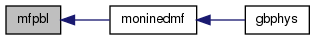
Referenced by moninedmf().
| subroutine moninedmf | ( | integer | ix, |
| integer | im, | ||
| integer | km, | ||
| integer | ntrac, | ||
| integer | ntcw, | ||
| real(kind=kind_phys), dimension(im,km) | dv, | ||
| real(kind=kind_phys), dimension(im,km) | du, | ||
| real(kind=kind_phys), dimension(im,km) | tau, | ||
| real(kind=kind_phys), dimension(im,km,ntrac) | rtg, | ||
| real(kind=kind_phys), dimension(ix,km) | u1, | ||
| real(kind=kind_phys), dimension(ix,km) | v1, | ||
| real(kind=kind_phys), dimension(ix,km) | t1, | ||
| real(kind=kind_phys), dimension(ix,km,ntrac) | q1, | ||
| real(kind=kind_phys), dimension(ix,km) | swh, | ||
| real(kind=kind_phys), dimension(ix,km) | hlw, | ||
| real(kind=kind_phys), dimension(im) | xmu, | ||
| real(kind=kind_phys), dimension(im) | psk, | ||
| real(kind=kind_phys), dimension(im) | rbsoil, | ||
| real(kind=kind_phys), dimension(im) | zorl, | ||
| real(kind=kind_phys), dimension(im) | u10m, | ||
| real(kind=kind_phys), dimension(im) | v10m, | ||
| real(kind=kind_phys), dimension(im) | fm, | ||
| real(kind=kind_phys), dimension(im) | fh, | ||
| real(kind=kind_phys), dimension(im) | tsea, | ||
| real(kind=kind_phys), dimension(im) | qss, | ||
| real(kind=kind_phys), dimension(im) | heat, | ||
| real(kind=kind_phys), dimension(im) | evap, | ||
| real(kind=kind_phys), dimension(im) | stress, | ||
| real(kind=kind_phys), dimension(im) | spd1, | ||
| integer, dimension(im) | kpbl, | ||
| real(kind=kind_phys), dimension(ix,km+1) | prsi, | ||
| real(kind=kind_phys), dimension(ix,km) | del, | ||
| real(kind=kind_phys), dimension(ix,km) | prsl, | ||
| real(kind=kind_phys), dimension(ix,km) | prslk, | ||
| real(kind=kind_phys), dimension(ix,km+1) | phii, | ||
| real(kind=kind_phys), dimension(ix,km) | phil, | ||
| real(kind=kind_phys) | delt, | ||
| logical | dspheat, | ||
| real(kind=kind_phys), dimension(im) | dusfc, | ||
| real(kind=kind_phys), dimension(im) | dvsfc, | ||
| real(kind=kind_phys), dimension(im) | dtsfc, | ||
| real(kind=kind_phys), dimension(im) | dqsfc, | ||
| real(kind=kind_phys), dimension(im) | hpbl, | ||
| real(kind=kind_phys), dimension(im) | hgamt, | ||
| real(kind=kind_phys), dimension(im) | hgamq, | ||
| real(kind=kind_phys), dimension(im,km-1) | dkt, | ||
| integer, dimension(im) | kinver, | ||
| real(kind=kind_phys) | xkzm_m, | ||
| real(kind=kind_phys) | xkzm_h, | ||
| real(kind=kind_phys) | xkzm_s, | ||
| logical | lprnt, | ||
| integer | ipr | ||
| ) |
This subroutine contains all of logic for the Hybrid EDMF PBL scheme except for the calculation of the updraft properties and mass flux.
The scheme works on a basic level by calculating background diffusion coefficients and updating them according to which processes are occurring in the column. The most important difference in diffusion coefficients occurs between those levels in the PBL and those above the PBL, so the PBL height calculation is of utmost importance. An initial estimate is calculated in a "predictor" step in order to calculate Monin-Obukhov similarity values and a corrector step recalculates the PBL height based on updated surface thermal characteristics. Using the PBL height and the similarity parameters, the diffusion coefficients are updated below the PBL top based on Hong and Pan (1996) [26] (including counter-gradient terms). Diffusion coefficients in the free troposphere (above the PBL top) are calculated according to Louis (1979) [40] with updated Richardson number-dependent functions. If it is diagnosed that PBL top-down mixing is occurring according to Lock et al. (2000) [38] , then then diffusion coefficients are updated accordingly. Finally, for convective boundary layers (defined as when the Obukhov length exceeds a threshold), the counter-gradient terms are replaced using the mass flux scheme of Siebesma et al. (2007) [49] . In order to return time tendencies, a fully implicit solution is found using tridiagonal matrices, and time tendencies are "backed out." Before returning, the time tendency of temperature is updated to reflect heating due to TKE dissipation following Han et al. (2015) [22] .
| [in] | ix | horizontal dimension |
| [in] | im | number of used points |
| [in] | km | vertical layer dimension |
| [in] | ntrac | number of tracers |
| [in] | ntcw | cloud condensate index in the tracer array |
| [in,out] | dv | v-momentum tendency ( \( m s^{-2} \)) |
| [in,out] | du | u-momentum tendency ( \( m s^{-2} \)) |
| [in,out] | tau | temperature tendency ( \( K s^{-1} \)) |
| [in,out] | rtg | moisture tendency ( \( kg kg^{-1} s^{-1} \)) |
| [in] | u1 | u component of layer wind ( \( m s^{-1} \)) |
| [in] | v1 | v component of layer wind ( \( m s^{-1} \)) |
| [in] | t1 | layer mean temperature ( \( K \)) |
| [in] | q1 | layer mean tracer concentration (units?) |
| [in] | swh | total sky shortwave heating rate ( \( K s^-1 \)) |
| [in] | hlw | total sky longwave heating rate ( \( K s^-1 \)) |
| [in] | xmu | time step zenith angle adjust factor for shortwave |
| [in] | psk | Exner function at surface interface? |
| [in] | rbsoil | surface bulk Richardson number |
| [in] | zorl | surface roughness (units?) |
| [in] | u10m | 10-m u wind ( \( m s^{-1} \)) |
| [in] | v10m | 10-m v wind ( \( m s^{-1} \)) |
| [in] | fm | fm parameter from PBL scheme |
| [in] | fh | fh parameter from PBL scheme |
| [in] | tsea | ground surface temperature (K) |
| [in] | qss | surface saturation humidity (units?) |
| [in] | heat | surface sensible heat flux (units?) |
| [in] | evap | evaporation from latent heat flux (units?) |
| [in] | stress | surface wind stress? ( \( cm*v^2\) in sfc_diff subroutine) (units?) |
| [in] | spd1 | surface wind speed? (units?) |
| [out] | kpbl | PBL top index |
| [in] | prsi | pressure at layer interfaces (units?) |
| [in] | del | pressure difference between level k and k+1 (units?) |
| [in] | prsl | mean layer pressure (units?) |
| [in] | prslk | Exner function at layer |
| [in] | phii | interface geopotential height (units?) |
| [in] | phil | layer geopotential height (units?) |
| [in] | delt | physics time step (s) |
| [in] | dspheat | flag for TKE dissipative heating |
| [out] | dusfc | surface u-momentum tendency (units?) |
| [out] | dvsfc | surface v-momentum tendency (units?) |
| [out] | dtsfc | surface temperature tendency (units?) |
| [out] | dqsfc | surface moisture tendency (units?) |
| [out] | hpbl | PBL top height (m) |
| [out] | hgamt | counter gradient mixing term for temperature (units?) |
| [out] | hgamq | counter gradient mixing term for moisture (units?) |
| [out] | dkt | diffusion coefficient for temperature (units?) |
| [in] | kinver | index location of temperature inversion |
| [in] | xkzm_m | background vertical diffusion coefficient for momentum (units?) |
| [in] | xkzm_h | background vertical diffusion coefficeint for heat, moisture (units?) |
| [in] | xkzm_s | sigma threshold for background momentum diffusion (units?) |
| [in] | lprnt | flag to print some output |
| [in] | ipr | index of point to print |
The calculation of the boundary layer height follows Troen and Mahrt (1986) [53] section 3. The approach is to find the level in the column where a modified bulk Richardson number exceeds a critical value.
The temperature of the thermal is of primary importance. For the initial estimate of the PBL height, the thermal is assumed to have one of two temperatures. If the boundary layer is stable, the thermal is assumed to have a temperature equal to the surface virtual temperature. Otherwise, the thermal is assumed to have the same virtual potential temperature as the lowest model level. For the stable case, the critical bulk Richardson number becomes a function of the wind speed and roughness length, otherwise it is set to a tunable constant.
Given the thermal's properties and the critical Richardson number, a loop is executed to find the first level above the surface where the modified Richardson number is greater than the critical Richardson number, using equation 10a from Troen and Mahrt (1986) [53] (also equation 8 from Hong and Pan (1996) [26]):
\[ h = Ri\frac{T_0\left|\vec{v}(h)\right|^2}{g\left(\theta_v(h) - \theta_s\right)} \]
where \(h\) is the PBL height, \(Ri\) is the Richardson number, \(T_0\) is the virtual potential temperature near the surface, \(\left|\vec{v}\right|\) is the wind speed, and \(\theta_s\) is for the thermal. Rearranging this equation to calculate the modified Richardson number at each level, k, for comparison with the critical value yields:
\[ Ri_k = gz(k)\frac{\left(\theta_v(k) - \theta_s\right)}{\theta_v(1)*\vec{v}(k)} \]
Once the level is found, some linear interpolation is performed to find the exact height of the boundary layer top (where \(Ri = Ri_{cr}\)) and the PBL height and the PBL top index are saved (hpblx and kpblx, respectively)
Using the initial guess for the PBL height, Monin-Obukhov similarity parameters are calculated. They are needed to refine the PBL height calculation and for calculating diffusion coefficients.
First, calculate the Monin-Obukhov nondimensional stability parameter, commonly referred to as \(\zeta\) using the following equation from Businger et al. (1971) [6] (equation 28):
\[ \zeta = Ri_{sfc}\frac{F_m^2}{F_h} = \frac{z}{L} \]
where \(F_m\) and \(F_h\) are surface Monin-Obukhov stability functions calculated in sfc_diff.f and \(L\) is the Obukhov length. Then, the nondimensional gradients of momentum and temperature (phim and phih) are calculated using equations 5 and 6 from Hong and Pan (1996) [26] depending on the surface layer stability. Then, the velocity scale valid for the surface layer ( \(w_s\), wscale) is calculated using equation 3 from Hong and Pan (1996) [26]. For the neutral and unstable PBL above the surface layer, the convective velocity scale, \(w_*\), is calculated according to:
\[ w_* = \left(\frac{g}{\theta_0}h\overline{w'\theta_0'}\right)^{1/3} \]
and the mixed layer velocity scale is then calculated with equation 6 from Troen and Mahrt (1986) [53]
\[ w_s = (u_*^3 + 7\epsilon k w_*^3)^{1/3} \]
Next, the counter-gradient terms for temperature and humidity are calculated using equation 4 of Hong and Pan (1996) [26] and are used to calculate the "scaled virtual temperature excess near the surface" (equation 9 in Hong and Pan (1996) [26]) so that the properties of the thermal are updated to recalculate the PBL height.
The PBL height calculation follows the same procedure as the predictor step, except that it uses an updated virtual potential temperature for the thermal.
For an unstable PBL, the Prandtl number is calculated according to Hong and Pan (1996) [26], equation 10, whereas for a stable boundary layer, the Prandtl number is simply \(Pr = \frac{\phi_h}{\phi_m}\).
Below the PBL top, the diffusion coefficients ( \(K_m\) and \(K_h\)) are calculated according to equation 2 in Hong and Pan (1996) [26] where a different value for \(w_s\) (PBL vertical velocity scale) is used depending on the PBL stability. \(K_h\) is calculated from \(K_m\) using the Prandtl number. The calculated diffusion coefficients are checked so that they are bounded by maximum values and the local background diffusion coefficients.
Diffusion coefficients above the PBL top are computed as a function of local stability (gradient Richardson number), shear, and a length scale from Louis (1979) [40] :
\[ K_{m,h}=l^2f_{m,h}(Ri_g)\left|\frac{\partial U}{\partial z}\right| \]
The functions used ( \(f_{m,h}\)) depend on the local stability. First, the gradient Richardson number is calculated as
\[ Ri_g=\frac{\frac{g}{T}\frac{\partial \theta_v}{\partial z}}{\frac{\partial U}{\partial z}^2} \]
where \(U\) is the horizontal wind. For the unstable case ( \(Ri_g < 0\)), the Richardson number-dependent functions are given by
\[ f_h(Ri_g) = 1 + \frac{8\left|Ri_g\right|}{1 + 1.286\sqrt{\left|Ri_g\right|}}\\ \]
\[ f_m(Ri_g) = 1 + \frac{8\left|Ri_g\right|}{1 + 1.746\sqrt{\left|Ri_g\right|}}\\ \]
For the stable case, the following formulas are used
\[ f_h(Ri_g) = \frac{1}{\left(1 + 5Ri_g\right)^2}\\ \]
\[ Pr = \frac{K_h}{K_m} = 1 + 2.1Ri_g \]
The source for the formulas used for the Richardson number-dependent functions is unclear. They are different than those used in Hong and Pan (1996) [26] as the previous documentation suggests. They follow equation 14 of Louis (1979) [40] for the unstable case, but it is unclear where the values of the coefficients \(b\) and \(c\) from that equation used in this scheme originate. Finally, the length scale, \(l\) is calculated according to the following formula from Hong and Pan (1996) [26]
\[ \frac{1}{l} = \frac{1}{kz} + \frac{1}{l_0}\\ \]
\[ or\\ \]
\[ l=\frac{l_0kz}{l_0+kz} \]
where \(l_0\) is currently 30 m for stable conditions and 150 m for unstable. Finally, the diffusion coefficients are kept in a range bounded by the background diffusion and the maximum allowable values.
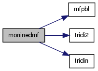
If the PBL is convective, the updraft properties are initialized to be the same as the state variables and the subroutine mfpbl is called.
For details of the mfpbl subroutine, step into its documentation mfpbl
If a stratocumulus layer has been identified in the PBL, the diffusion coefficients in the PBL are modified in the following way.
\[ K_h^{Sc} = -c\frac{\Delta F_R}{\rho c_p}\frac{1}{\frac{\partial \theta_v}{\partial z}} \]
where the constant \(c\) is set to 0.2 if the CTEI criterion is not met and 1.0 if it is.After \(K_h^{Sc}\) has been determined from the surface to the top of the stratocumulus layer, it is added to the value for the diffusion coefficient calculated previously using surface-based mixing [see equation 6 of Lock et al. (2000) [38] ].
The tendencies of heat, moisture, and momentum due to vertical diffusion are calculated using a two-part process. First, a solution is obtained using an implicit time-stepping scheme, then the time tendency terms are "backed out". The tridiagonal matrix elements for the implicit solution for temperature and moisture are prepared in this section, with differing algorithms depending on whether the PBL was convective (substituting the mass flux term for counter-gradient term), unstable but not convective (using the computed counter-gradient terms), or stable (no counter-gradient terms).
The tridiagonal system is solved by calling the internal tridin subroutine.
After returning with the solution, the tendencies for temperature and moisture are recovered.
Following Han et al. (2015) [22] , turbulence dissipation contributes to the tendency of temperature in the following way. First, turbulence dissipation is calculated by equation 17 of Han et al. (2015) [22] for the PBL and equation 16 for the surface layer.
Next, the temperature tendency is updated following equation 14.
As with the temperature and moisture tendencies, the horizontal momentum tendencies are calculated by solving tridiagonal matrices after the matrices are prepared in this section.
Finally, the tendencies are recovered from the tridiagonal solutions.
Definition at line 96 of file moninedmf.f.
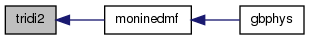
References physcons::con_cp, physcons::con_g, physcons::con_hvap, physcons::con_rd, mfpbl(), tridi2(), and tridin().
Referenced by gbphys().

| subroutine tridi2 | ( | integer | l, |
| integer | n, | ||
| real(kind=kind_phys), dimension(l,2:n) | cl, | ||
| real(kind=kind_phys), dimension(l,n) | cm, | ||
| real(kind=kind_phys), dimension(l,n-1) | cu, | ||
| real(kind=kind_phys), dimension(l,n) | r1, | ||
| real(kind=kind_phys), dimension(l,n) | r2, | ||
| real(kind=kind_phys), dimension(l,n-1) | au, | ||
| real(kind=kind_phys), dimension(l,n) | a1, | ||
| real(kind=kind_phys), dimension(l,n) | a2 | ||
| ) |
Routine to solve the tridiagonal system to calculate temperature and moisture at \( t + \Delta t \); part of two-part process to calculate time tendencies due to vertical diffusion.
Origin of subroutine unknown.
Definition at line 1196 of file moninedmf.f.
Referenced by moninedmf().
| subroutine tridin | ( | integer | l, |
| integer | n, | ||
| integer | nt, | ||
| real(kind=kind_phys), dimension(l,2:n) | cl, | ||
| real(kind=kind_phys), dimension(l,n) | cm, | ||
| real(kind=kind_phys), dimension(l,n-1) | cu, | ||
| real(kind=kind_phys), dimension(l,n) | r1, | ||
| real(kind=kind_phys), dimension(l,n*nt) | r2, | ||
| real(kind=kind_phys), dimension(l,n-1) | au, | ||
| real(kind=kind_phys), dimension(l,n) | a1, | ||
| real(kind=kind_phys), dimension(l,n*nt) | a2 | ||
| ) |
Routine to solve the tridiagonal system to calculate u- and v-momentum at \( t + \Delta t \); part of two-part process to calculate time tendencies due to vertical diffusion.
Origin of subroutine unknown.
Definition at line 1239 of file moninedmf.f.
Referenced by moninedmf().
 1.8.10